Introduction
Alright, let's talk probability. It might sound like something from a dusty old textbook, but you literally use it every day. Deciding if you should risk texting in class? That's probability. Wondering about the drop rate for that legendary skin in your favorite game? Probability. It's just the math behind chance. We're going to break it down so you can predict outcomes better than a TikTok trend predictor. Let's get this! 💪
Understanding the Probability ScaleC8.1
Think of probability as a scale from 0 to 1. If something has a probability of 0, it's impossible (like your parents suddenly loving your loud music). If it has a probability of 1, it's certain (like getting a notification on your phone in the next hour). Everything else—like passing your driving test first time—is somewhere in between. We can write probabilities as fractions, decimals, or percentages. 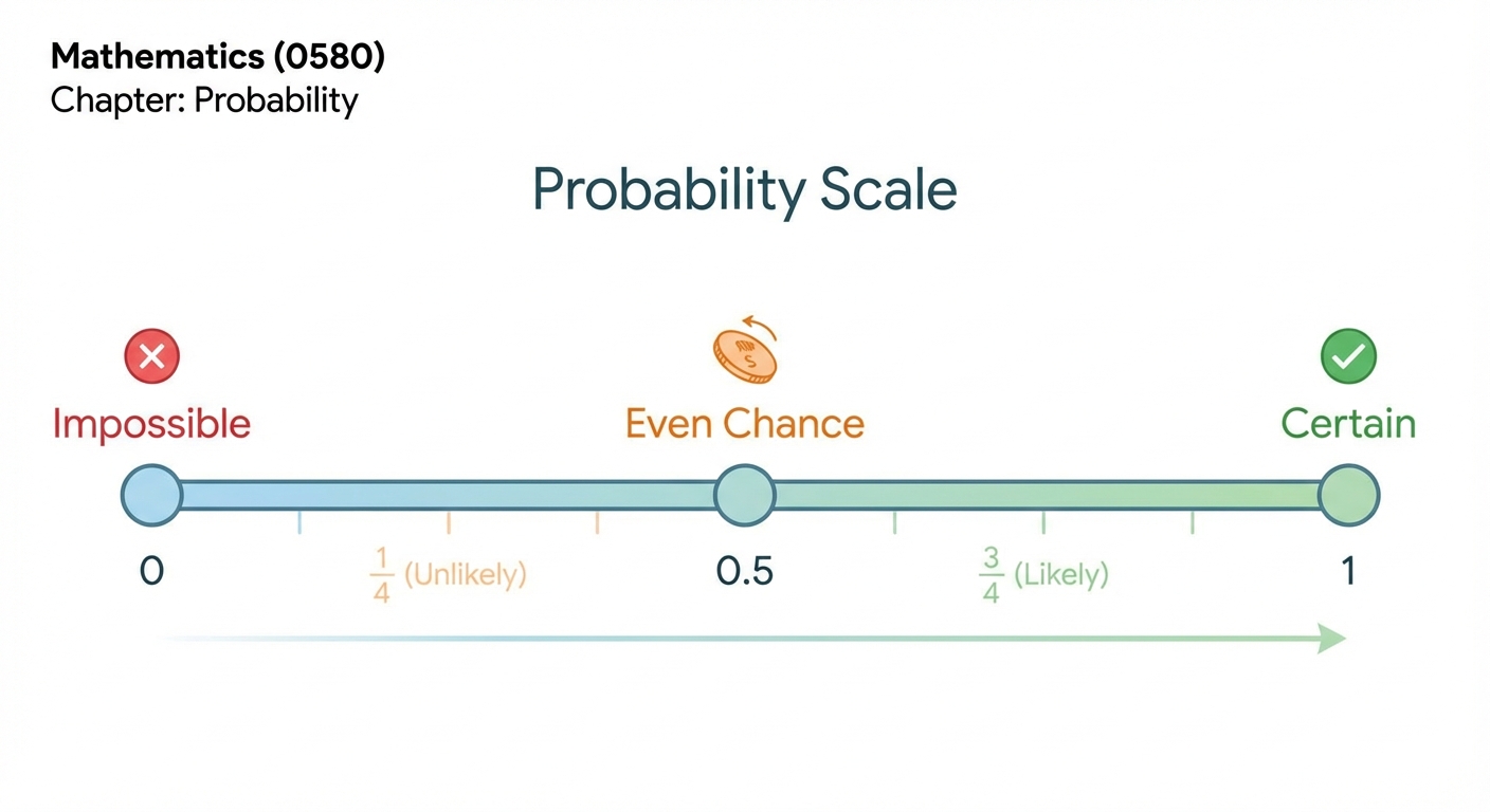
Worked Example: Calculating Simple ProbabilityC8.1
Problem A bag contains 5 red, 3 blue, and 2 green marbles. What is the probability of picking a blue marble at random?
Step 1 First, find the total number of possible outcomes. This is just the total number of marbles in the bag. $$5 + 3 + 2 = 10 \text{ total marbles}$$
Step 2 Next, identify the number of favourable outcomes. We want to pick a blue marble, and there are 3 of them. $$\text{Favourable outcomes (blue)} = 3$$
Step 3 The probability is the number of favourable outcomes divided by the total number of outcomes. Always simplify the fraction if you can! $$P(\text{blue}) = \frac{\text{Number of blue marbles}}{\text{Total number of marbles}} = \frac{3}{10}$$
The Complement Rule: Probability of an Event Not OccurringC8.1
This one's a super useful shortcut. Sometimes it's easier to figure out the probability of something not happening. Since the total probability of all outcomes is always 1 (or 100%), the probability of an event not occurring is just 1 minus the probability that it does occur. Think of it like this: if the chance of rain is 30% ($0.3$), the chance of it not raining is 100% - 30% = 70% ($0.7$). The formula is your new best friend: $P(A') = 1 - P(A)$.
Worked Example: Applying the Complement RuleC8.1
Problem The probability of your favourite football team winning their next match is $0.65$. What is the probability that they do not win?
Step 1 We know the total probability of all outcomes (win, lose, or draw) must be 1. We are given the probability of winning. $$P(\text{win}) = 0.65$$
Step 2 To find the probability of them not winning, we use the rule $P(\text{not A}) = 1 - P(\text{A})$. In this case, 'not winning' covers both losing and drawing. $$P(\text{not win}) = 1 - P(\text{win}) = 1 - 0.65 = 0.35$$
Theoretical vs. Experimental ProbabilityC8.2
Theoretical probability is what we expect to happen. For a fair coin, we expect heads 50% of the time. But what if you flip it 10 times and get 7 heads? That's experimental probability or relative frequency. It's what actually happened in your experiment. The more you repeat an experiment (like, flipping the coin 1000 times), the closer your relative frequency will get to the theoretical probability. It's like checking the vibe of a situation based on what's actually going down, not just what you thought would happen.
Worked Example: Calculating Relative FrequencyC8.2
Problem You work a part-time job at a cafe. You record the hot drinks sold one morning: 40 coffees, 25 teas, and 15 hot chocolates. What is the relative frequency of a customer ordering a tea?
Step 1 First, find the total number of trials, which is the total number of drinks sold. $$\text{Total trials} = 40 + 25 + 15 = 80$$
Step 2 The relative frequency is the number of times the event occurred (tea was sold) divided by the total number of trials. $$\text{Relative Frequency (Tea)} = \frac{\text{Frequency of event}}{\text{Total trials}} = \frac{25}{80}$$
Step 3 Simplify the fraction for your final answer. Both numbers are divisible by 5. $$\frac{25}{80} = \frac{5}{16}$$
Calculating Expected Frequency from Theoretical ProbabilityC8.2
Okay, this is where probability gets powerful. Expected frequency is your best guess at how many times something will happen over a bunch of trials. Think of it like a prediction. If you know the probability of an event, you can predict how often it'll occur. The formula is simple: Expected Frequency = (number of trials) $\times$ (probability of the event). We'll call the number of trials '$n$' to look official. So, $E = n \times p$.
Worked Example: Calculating Expected FrequencyC8.2
Problem A fair six-sided die is rolled 300 times. How many times would you expect to roll a 5?
Step 1 First, find the theoretical probability of the event. There is one '5' on a die with six faces. $$P(5) = \frac{1}{6}$$
Step 2 Next, identify the number of trials ($n$). The problem states the die is rolled 300 times. $$n = 300$$
Step 3 Now, use the formula: Expected Frequency = $n \times p$. Multiply the number of trials by the probability of the event. $$\text{Expected number of 5s} = 300 \times \frac{1}{6} = \frac{300}{6} = 50$$
Calculating Expected Frequency Using Relative FrequencyC8.2
What if you don't know the theoretical probability? Maybe you have a biased spinner or a dodgy die from a cheap board game. This is where your experimental data (relative frequency) comes in clutch. You can use the relative frequency from a past experiment as your best estimate for the probability. Then, you use the same expected frequency formula, just subbing in your relative frequency for '$p$'. This is how companies predict sales based on past data!
Worked Example: Expected Frequency from Relative FrequencyC8.2
Problem A spinner is spun 200 times. It lands on Red 80 times. If the spinner is spun another 50 times, how many times would you expect it to land on Red?
Step 1 First, calculate the relative frequency (our estimate of probability) from the first experiment. $$P(\text{Red}) \approx \text{Relative Frequency} = \frac{80}{200} = \frac{2}{5} \text{ or } 0.4$$
Step 2 Now use this probability to predict the outcome for the next set of trials. The number of new trials is 50. $$\text{Expected Frequency} = n \times p = 50 \times 0.4$$
Step 3 Calculate the final answer. You'd expect it to land on Red 20 times. $$50 \times 0.4 = 20$$
The Sum of Probabilities for All OutcomesC8.3
This is a quick but important one. For any event, the sum of the probabilities of all possible outcomes must equal 1. If a spinner can land on Red, Blue, or Green, then $P(\text{Red}) + P(\text{Blue}) + P(\text{Green}) = 1$. This is super helpful for finding a missing probability if you know the others. 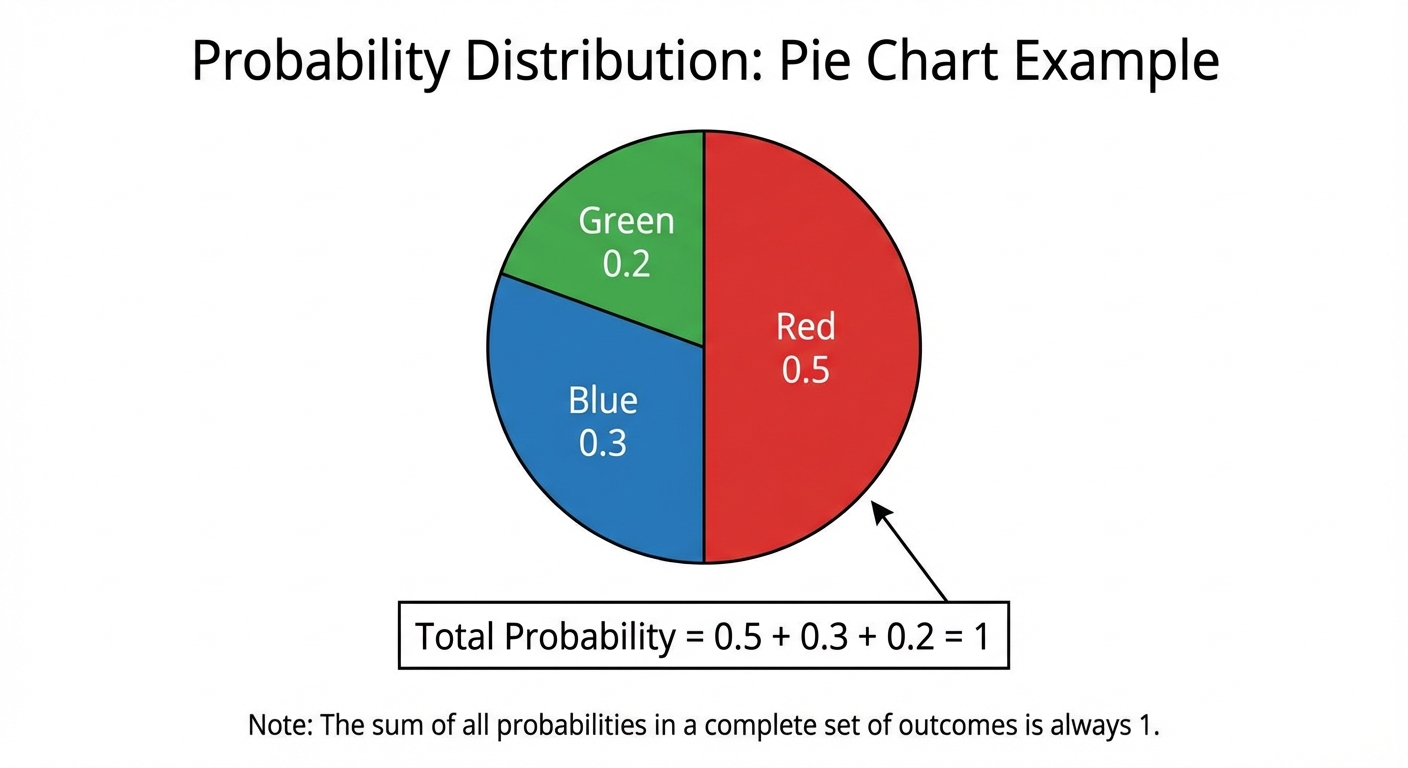
Worked Example: Finding a Missing ProbabilityC8.1
Problem The probability of a bus being early is 0.1, and the probability of it being on time is 0.65. What is the probability of it being late? (Assuming these are the only three outcomes).
Step 1 We know the probabilities of all possible outcomes must add up to 1. $$P(\text{early}) + P(\text{on time}) + P(\text{late}) = 1$$
Step 2 Add the probabilities we already know. $$0.1 + 0.65 = 0.75$$
Step 3 Subtract this sum from 1 to find the missing probability of the bus being late. $$P(\text{late}) = 1 - 0.75 = 0.25$$
Single Event Probability and the Probability ScaleC8.1
Okay, so life is full of 'maybes'. Will you pass your driving test? Will your favourite artist drop a surprise album? Probability is just the cool mathematical way of putting a number on that 'maybe'. Think of it like a scale, or a slider, that goes from 0 to 1. 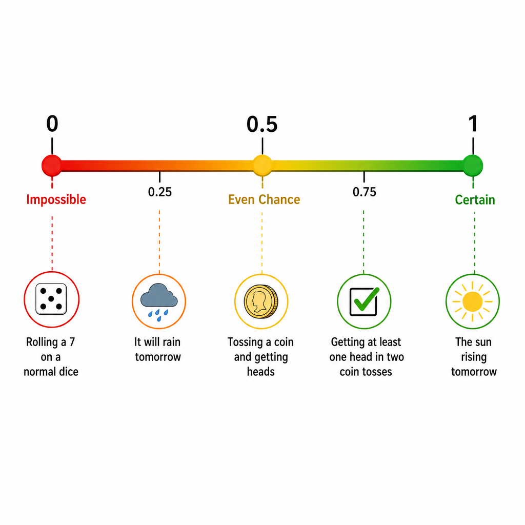 A probability of 0 means the event is impossible – like getting a legendary skin from your first-ever loot box. A probability of 1 means it's certain to happen – like getting a new Snapchat notification in the next hour. A 0.5 is a perfect 50/50 even chance, like a coin toss.<br><br>To calculate the probability of a single event, we use a straightforward formula: $$P(\text{Event}) = \frac{\text{Number of favourable outcomes}}{\text{Total number of possible outcomes}}$$ 'Favourable outcomes' is just a fancy way of saying 'the outcomes you want to happen'. 'Total outcomes' is everything that could possibly happen. For example, the probability of rolling a 5 on a standard six-sided dice is $\frac{1}{6}$ because there's only one '5' (favourable) out of six possible numbers (total). You can write your answer as a fraction ($\frac{1}{6}$), a decimal ($\approx 0.167$), or a percentage ($\approx 16.7\%$).<br><br>Finally, let's talk about the 'not' rule. Sometimes it's easier to figure out the chance of something not happening. The rule is simple: $$P(\text{not A}) = 1 - P(\text{A})$$ Since the total probability of all outcomes is 1 (certainty), you just subtract the probability of the event you're interested in. So, the probability of not rolling a 5 is $1 - \frac{1}{6} = \frac{5}{6}$. It's a super useful shortcut!
Worked Example: Calculating Probability from a TableC8.1
Problem You're working at a cafe and the manager has a fixed playlist of 80 songs on shuffle. The genres are: 45 Pop songs, 20 Hip-Hop songs, and 15 Indie songs. If a song is picked at random, what is the probability that it is not a Pop song? Give your answer as a fraction in its simplest form.
Step 1 First, let's confirm the total number of outcomes. This is the total number of songs on the playlist, which the problem gives us, but it's always good to check the numbers add up! $$\text{Total songs} = 45 (\text{Pop}) + 20 (\text{Hip-Hop}) + 15 (\text{Indie}) = 80$$
Step 2 The question asks for the probability of the song not being Pop. The easiest way to solve this is to first find the probability that the song is Pop, and then use our 'not' rule. $$P(\text{Pop}) = \frac{\text{Number of Pop songs}}{\text{Total number of songs}} = \frac{45}{80}$$
Step 3 It's always best to simplify your fractions. We can see that both 45 and 80 are divisible by 5. Let's simplify P(Pop). $$\frac{45 \div 5}{80 \div 5} = \frac{9}{16}$$
Step 4 Now we apply the 'not' rule: $P(\text{not Pop}) = 1 - P(\text{Pop})$. This will give us our final answer. $$P(\text{not Pop}) = 1 - \frac{9}{16} = \frac{16}{16} - \frac{9}{16} = \frac{7}{16}$$
Step 5 Alternative Check: We could also find the number of non-Pop songs first (Hip-Hop + Indie) and calculate the probability directly. This is a great way to check your work! $$\text{Non-Pop songs} = 20 + 15 = 35 <br> P(\text{not Pop}) = \frac{35}{80} = \frac{7}{16}$$
Experimental Probability and Relative FrequencyC8.2
Okay, so we've all heard that if you flip a coin, there's a 50/50 chance of getting heads. That's theoretical probability – it's what should happen in a perfect world. But let's be real, life isn't perfect. Experimental probability is all about what actually happens when you run the experiment. It's the probability based on real data, not just theory.<br><br>The key term here is relative frequency. It's basically the same thing as experimental probability. Think of it as the event's 'score' from your experiment. The formula is super simple: $$ \text{Relative Frequency} = \frac{\text{Number of times an event happens}}{\text{Total number of trials}} $$ So, if you're trying to master a trick in a video game and you succeed 10 times out of 40 attempts, the relative frequency of you succeeding is $\frac{10}{40}$ or $0.25$. This number is your estimate of the probability. The cool part? The more you practice (i.e., the more trials you do), the more accurate this estimate becomes. It's like how a music streaming algorithm gets better at recommending songs the more you listen. 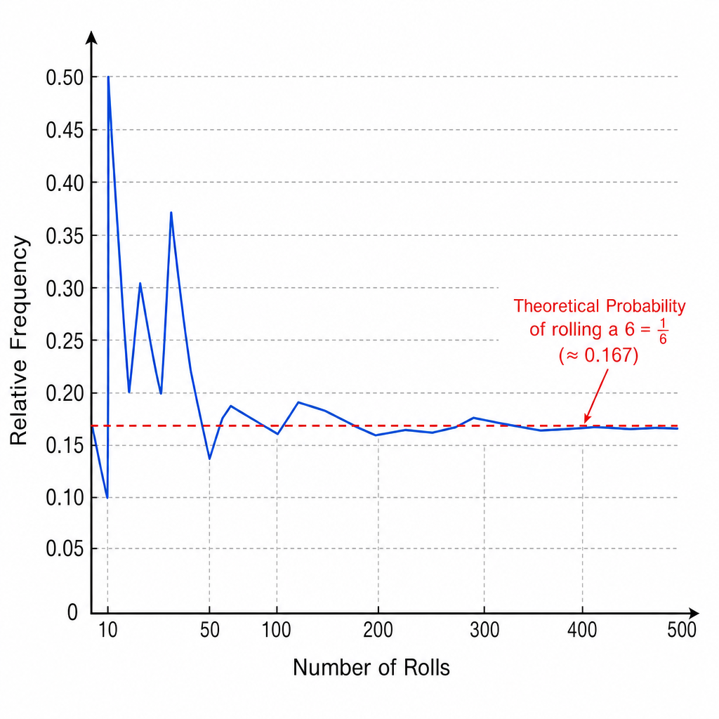 <br><br>This is also how we spot if something is biased. If a die is 'fair', each number has an equal chance. But if it's weighted or damaged, it's biased. If you roll it 100 times and get a '5' way more often than the other numbers, your experimental data (the relative frequencies) is telling you something's up. Finally, we can use this data to predict the future with expected frequency. If your boss at your weekend job knows that, based on last month's data, 20 per cent of customers buy a drink, you can expect how many will buy a drink out of the next 50 customers. The formula is: $$ \text{Expected Frequency} = \text{Probability} \times \text{Number of trials} $$ It's a powerful tool for making predictions based on what's happened before. It’s basically using the past to get a sneak peek at the future. 😉
Worked Example: Calculating Relative and Expected FrequencyC8.2
Problem Kenji suspects his four-sided spinner is biased. He spins it 200 times and records the results: <br>Red: 84<br>Blue: 46<br>Green: 52<br>Yellow: 18<br><br>a) What is the relative frequency of the spinner landing on Red?<br>b) If Kenji spins the spinner another 50 times, how many times would you expect it to land on Red?
Step 1 For part (a), we need to find the relative frequency (our experimental probability) for landing on Red. We use the formula: number of successful outcomes divided by the total number of trials. $$ \text{Relative Frequency (Red)} = \frac{\text{Number of times it landed on Red}}{\text{Total number of spins}} $$
Step 2 Now we plug in the numbers from Kenji's experiment. He spun it 200 times in total, and it landed on Red 84 of those times. $$ \text{Relative Frequency (Red)} = \frac{84}{200} = 0.42 $$
Step 3 So, the relative frequency of landing on Red is 0.42 or 42%. Because this is much higher than the theoretical probability for a fair four-sided spinner (which would be $\frac{1}{4} = 0.25$), Kenji is right to suspect it's biased! $$ P(\text{Red}) \approx 0.42 $$
Step 4 For part (b), we need to calculate the expected frequency. We'll use our experimental probability from part (a) to predict the outcome for the next 50 spins. The formula is Probability × New Number of Trials. $$ \text{Expected Frequency} = P(\text{Red}) \times \text{New number of spins} $$
Step 5 Let's substitute our values. We use our best estimate for the probability (0.42) and multiply it by the new number of trials (50). $$ \text{Expected Frequency} = 0.42 \times 50 = 21 $$
Step 6 So, based on his experiment, we would expect Kenji's spinner to land on Red about 21 times if he spins it another 50 times. It might not be exactly 21, but that's our most educated guess! $$ \text{Expected number of Reds} = 21 $$
Probability of Combined EventsC8.3
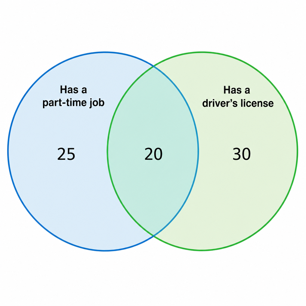
Alright, let's talk about combined events. Life isn't usually about just one thing happening, right? It's more like, what are the chances you'll ace your maths test and your favourite artist drops a surprise album on the same day? That's a combined event! It's simply the probability of two or more events happening together.<br><br>To figure this stuff out, we have a few awesome visual tools. First up is the sample space diagram. Think of this like a grid that shows every single possible outcome when two things happen. For example, if you roll two dice while playing a game, the sample space diagram would show all 36 possible combos, from (1,1) all the way to (6,6). It’s a super clear way to make sure you don't miss any possibilities. 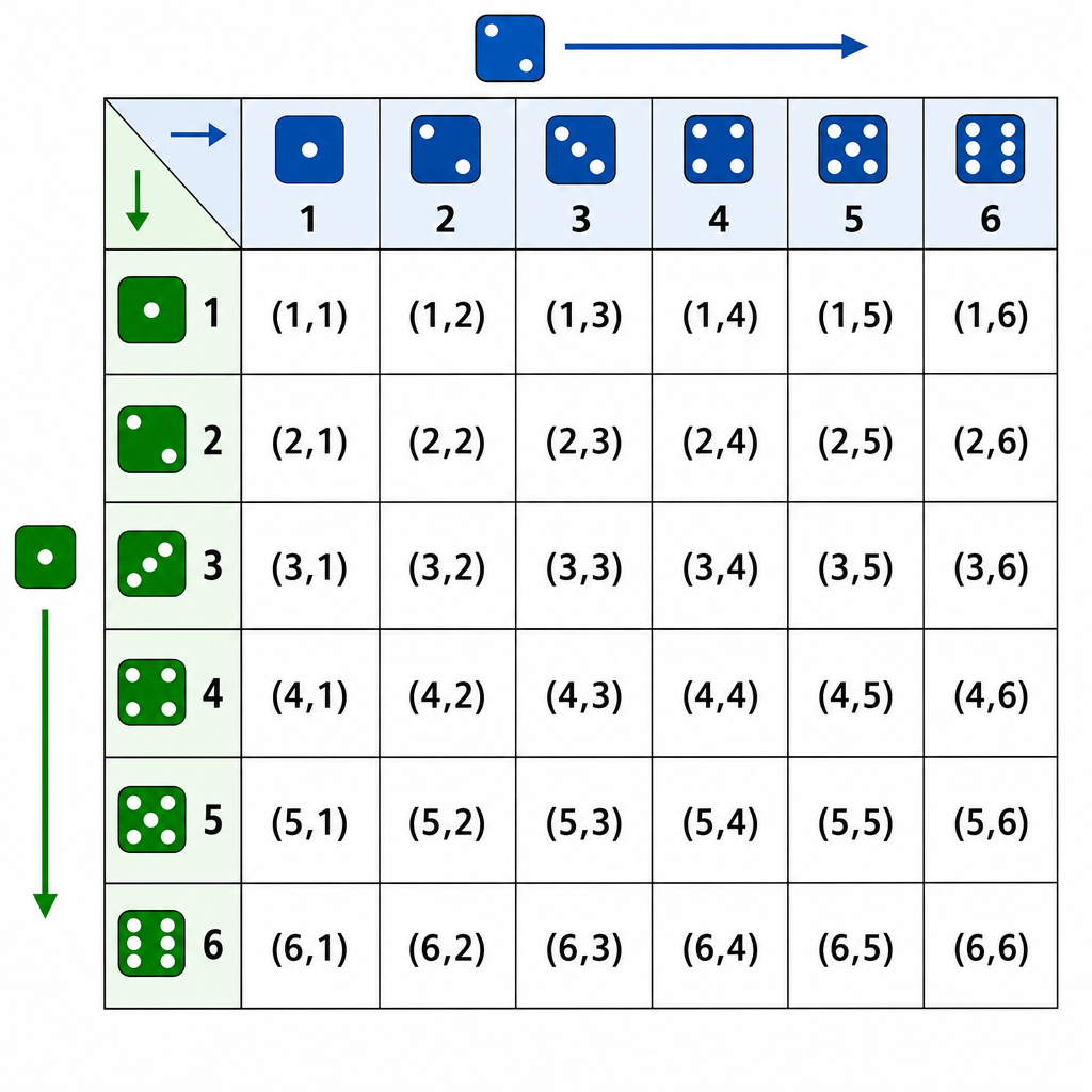 <br><br>Next, we have Venn diagrams. You've probably seen these before. They're perfect for showing overlap. Imagine one circle is 'Students who have a part-time job' and another is 'Students who have their driver's license'. The overlapping section shows the students who have both. For your exam, you'll only need to worry about two circles.
 <br><br>Finally, there's the tree diagram, which is like a 'choose your own adventure' map for probability. You start at one point, and branches split off for each possible outcome of the first event. Then, from the end of each of those branches, more branches split off for the second event. We write the probabilities on the branches and the final combined outcomes at the very end.
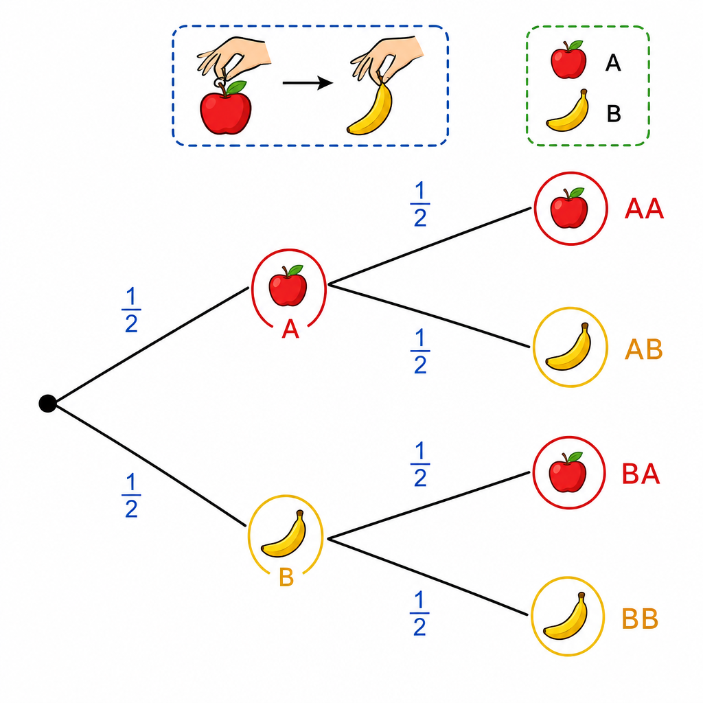 <br><br>Super important note: For IGCSE Core, we only deal with events with replacement. This means the situation resets after each event. It's like picking a song from a playlist; just because you heard it once doesn't mean it's removed. The total number of outcomes stays the same for the second event. Easy peasy! 👍
Worked Example: Using a Tree Diagram for Combined EventsC8.3
Problem In your wardrobe, you have 5 T-shirts: 3 are black (B) and 2 are white (W). You randomly pick a T-shirt to wear on Monday, then put it back. On Tuesday, you randomly pick another T-shirt. What is the probability that you pick a black T-shirt on both days?
Step 1 First, let's figure out the probabilities for a single pick. There are 5 T-shirts in total. The probability of picking a black one is the number of black shirts over the total. $$P(\text{Black}) = \frac{\text{Number of Black T-shirts}}{\text{Total T-shirts}} = \frac{3}{5}$$
Step 2 Similarly, let's find the probability of picking a white T-shirt. We'll need this to draw our full tree diagram. $$P(\text{White}) = \frac{\text{Number of White T-shirts}}{\text{Total T-shirts}} = \frac{2}{5}$$
Step 3 Now, let's set up the tree diagram for the two days. The first set of branches represents Monday's pick. The second set of branches represents Tuesday's pick. Since you put the T-shirt back ('with replacement'), the probabilities for Tuesday are exactly the same as for Monday. [This step is best visualized with a tree diagram. The first branches would be B (prob 3/5) and W (prob 2/5). From each of these, two more identical branches would extend.]
Step 4 We want to find the probability of picking a black T-shirt on both days. This corresponds to the 'Black-Black' (BB) path on our tree diagram. To find the probability of a combined path, we multiply the probabilities along the branches. $$P(\text{B and B}) = P(\text{B on Monday}) \times P(\text{B on Tuesday})$$
Step 5 Let's plug in the numbers and calculate the final probability. So, the chance of you rocking a black T-shirt two days in a row is 9 out of 25. $$P(\text{B and B}) = \frac{3}{5} \times \frac{3}{5} = \frac{9}{25}$$
Key Points to Remember 🎯
- Probability is measured on a scale from 0 (impossible) to 1 (certain).
- Simple Probability: $P(\text{event}) = \frac{\text{Number of favourable outcomes}}{\text{Total number of outcomes}}$
- The 'Not' Rule: $P(\text{not event}) = 1 - P(\text{event})$
- Relative Frequency (from an experiment): $\frac{\text{Frequency of event}}{\text{Total trials}}$
- Expected Frequency (prediction): $n \times P(\text{event})$, where $n$ is the number of trials.